BASSr Workflow

Packages and settings

library(dplyr)

## 
## Attaching package: 'dplyr'

## The following objects are masked from 'package:stats':
## 
##     filter, lag

## The following objects are masked from 'package:base':
## 
##     intersect, setdiff, setequal, union

library(ggplot2)
library(tidyr)
library(BASSr)
library(sf)

## Linking to GEOS 3.12.1, GDAL 3.8.4, PROJ 9.4.0; sf_use_s2() is TRUE

Introduction

The goal of this vignette is provide a guide from which to work from when implementing BASS into a survey design. There currently are quite a few peculiarities in the script and the workflow should elucidate them a bit more.

Step 1. Define your area of interest

For now I’ll work with the package sf’s nc layer. You will need to have the sf package installed (install.packages('sf')). We need a projection that usess metres instead of lat/lon so you may have to transform your spatial objects.

nc <- st_read(system.file("shape/nc.shp", package="sf")) %>% 
  st_transform(crs = '+proj=utm +zone=17 +ellps=GRS80 +units=m +no_defs ',check=T, partial=F)

## Reading layer `nc' from data source 
##   `/home/runner/work/_temp/Library/sf/shape/nc.shp' using driver `ESRI Shapefile'
## Simple feature collection with 100 features and 14 fields
## Geometry type: MULTIPOLYGON
## Dimension:     XY
## Bounding box:  xmin: -84.32385 ymin: 33.88199 xmax: -75.45698 ymax: 36.58965
## Geodetic CRS:  NAD27

nc_coords <- st_centroid(nc) %>% 
  st_coordinates %>% 
  as_tibble

## Warning: st_centroid assumes attributes are constant over geometries

nc_for_survey <- bind_cols(nc, nc_coords) %>% 
  filter(X < 600000)

We will just survey the western half of the state for simplicity (shown in grey).

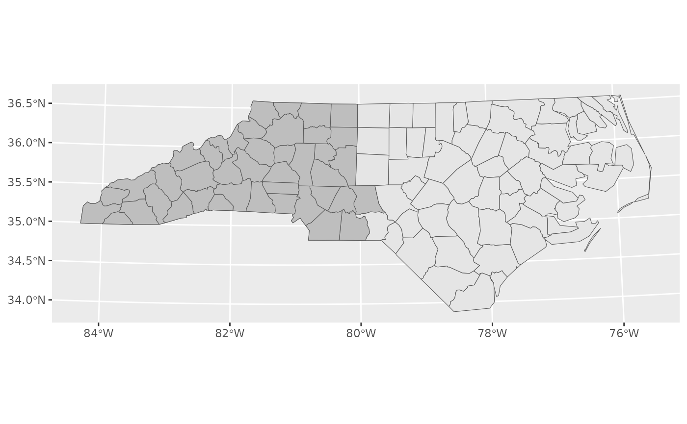
ggplot(nc) + geom_sf() + geom_sf(data = nc_for_survey, fill = 'grey')

For today, lets aim to survey North Carolina using 1km sample units and 34km study areas.

Step 2. Create hexagons

Often this is most usefully done outside of R, with habitat and costs incorporated into the hexagons, but I’ll run through it here to detail how the data should be formatted.

SA <- create_hexes(land = nc_for_survey,
                       hex_size =  100000, 
                      units = 'ha' )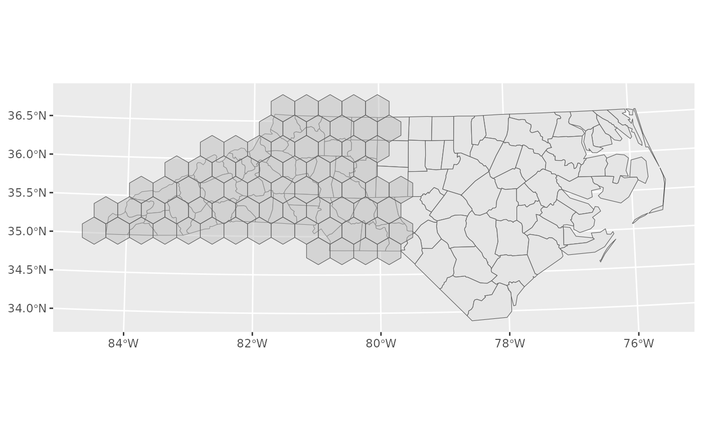

ggplot(SA) + 
  geom_sf(data = nc) + 
  geom_sf(fill = 'grey', alpha = 0.5)

Here is an example study area. Not all of the study area is within North Carolina (pink) and so we will not deploy here.

su_ex <- create_hexes(land = SA[16,],
                       hex_size =  100, 
                      units = 'ha' )

ggplot() +  
  geom_sf(data = nc, fill = 'lightpink') +
  geom_sf(data = SA[16,], fill = NA) +
  geom_sf(data = su_ex, fill = NA) +
  coord_sf(xlim =st_bbox(SA[16,])[c(1,3)], ylim = st_bbox(SA[16,])[c(2,4)])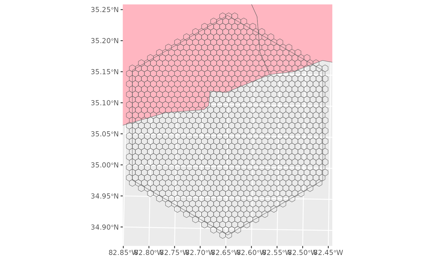

st_area(SA[16,])

## 1e+09 [m^2]

pHA_region <- tibble(lc = 1:18) %>% 
  mutate(pHA_region = runif(18),
         pHA_region = pHA_region/sum(pHA_region),
         varbeta = pHA_region*0.2)
# varbeta <- 0.2
estBetaParams <- function(mu, var) {
  alpha <- ((1 - mu) / var - 1 / mu) * mu ^ 2
  beta <- alpha * (1 / mu - 1)
  return(params = list(alpha = alpha, beta = beta))
}

beta_values <- estBetaParams(pHA_region$pHA_region, pHA_region$varbeta)
SA_LC <- 
expand_grid(hex_id = unique(SA$hex_id), lc = 1:18) %>% 
  left_join(pHA_region, by = 'lc') %>% 
  mutate(LandCover = glue::glue("LC{stringr::str_pad(lc,width = 2, side = 'left', pad = 0 )}"),
         pha = rbeta(nrow(.),beta_values$alpha,beta_values$beta)) %>% 
         # a = (pHA_region**2)*((1-pHA_region)/(varbeta)- (1/pHA_region)),
         # pha = rbeta(nrow(.),a,a*(1/pHA_region-1))) %>% 
  group_by(hex_id) %>% 
  mutate(ha = pha/sum(pha)*1e9*.0001,
         pha = ha/sum(ha)) %>% ungroup

David Hope

2025-06-20

Packages and settings

Introduction

Step 1. Define your area of interest

Step 2. Create hexagons