Cost Breakdown

knitr::opts_chunk$set(
  eval=T,
  collapse = TRUE,
  message =F, warning =F,
  fig.width = 8,
  fig.height = 8,
  comment = "#>"
)
library(dplyr)
library(purrr)
library(tidyr)
library(ggplot2)
library(sf)
library(BASSr)
library(patchwork)


bcv <- BASSr::cost_vars

Cost model parts

The cost model is comprised of three access types: * Truck * ATV * Helicopter

The basic cost is based on the number of ARUs to be deployed per study area ( $N$ ). The base rate is 30.

The cost of accessing a site is the sum of the cost of surveying a site by truck, atv and helicopter, each weighted by the proportion that is accessible by that access type. Truck access is assumed to be preffered first, then ATV, then helicopter.

$C = \sum p_iC_i = p_TC_T + p_AC_A + p_HC_H$

Truck access is based on primary roads plus a buffer of 1000m. A truck cost is based on the following formula.

$C_{T} = \frac{T_dn_c N}{N_Tn_c} = \frac{T_d N}{N_T}$ Where $T_d$ is the daily cost of truck usage, set initially to 600. $N_T$ is the number of ARUs a truck crew can deploy (5). This can be changed later to allow for differing daily costs based on the number of truck crews, however as written now, the number of crews ( $n_c$ ) increases deployment rate and cost equivanetly and therefore drops out of the equation.

The cost of ATV deployment is equivalent to truck costs in structure, but the rate of deployment and costs are different between deployment types: $C_{A} = \frac{A_dn_c N}{N_An_c} = \frac{A_d N}{N_A}$

The cost of helicopter deployment has more details. It can be broken down into four pieces: 1. The cost per litre of fuel - $C_l$ 2. The cost of setting up a basecamp - $C_b$ 3. The cost of moving to/from the study area - $C_{f}$ 4. The cost of moving within the study area - $C_{sa}$

The distances between the study area, basecamp and nearest airport drive most of the cost. The distance between the nearest airport and the study area is $D_{s-a}$ , between the study area and basecamp $D_{s-b}$ , and between basecamp and the airport $D_{a-b}$ . If the distance from the airport to the study area is less than a maximum helicopter range $D_{s-a}<D_{max}$ then a basecamp is not needed. If the distance from the basecamp to the study area is greater than $D_{max}$ , then a fuel cache is required. Adding a basecamp and fuel cache increase the cost per litre for the helicopter to fly.

$C_l = \begin{cases} C_l[1], & \text{if } D_{s-a} < D_{max} \\ C_l[2], & \text{else if } D_{s_b} < D_{max}\\ C_l[3], & \text{ otherwise} \end{cases}$

The cost of flying from the airport to the basecamp is as follows:

$C_b = \begin{cases} 0,& \text{if } D_{s-a} < D_{max} \\ D_{a-b} C^*_b + 2\frac{D_{a-b}}{S_h}l_hC_l, & \text{otherwise} \end{cases}$ where $C^*_b$ is the cost of setting up the basecamp per kilometre from an airport($9 $km^{-1}$ ), $S_h$ is the helicopter relocation speed in kilometres per hour (180 $km/hr$ ), and $l_h$ is the litres of fuel consumed per hour the helicopter is operational (160 $l/hr$ ).

In the next version we may want to put a cap based on crew size as the cost is capped by weight. So a further flight may require a smaller crew.

The cost of flying to the study area is: $C_{f} = \begin{cases} 2D_{s-a}C_D,& \text{if } D_{s-a} < D_{max} \\ 2D_{s-b}C_D, & \text{otherwise} \end{cases}$ where $C_D$ is the cost per kilometre: $C_D = \frac{l_hC_l + C_H}{S_h}$

The cost of operating within the study area is: $C_{sa} = N\frac{l_hC_l + C_H}{n_hN_h}H_f$ where $H_f$ is the hours flying within the study area per day, $n_h$ is the crew size, and $N_h$ is ARUs deployed per day per crew memeber.

The final cost for helicopter is: $C_H = C_{sa} + C_{f} + C_b$

How does this look in practice? Lets look at what deploying an increasing number of ARUs looks like for study areas with just 1 of the three deployment methods. Here I’ve set up a pretend study area that is intially 250km from the airport, 100km from the basecamp, and with 200km from the airport to the basecamp. I’ve then compared this to a study area with just roads, just atv roads, a study area not requiring a basecamp, a study area requiring a secondary fuel cache. I’ve also included a mixed study area that required 30% truck, ATV, and helicopter. We see how the cost changes with the number of ARUs deployed.

maxARUs <- 200
 d_heli <- tibble(StudyAreaID  = "Helicopter", 
        pr= 0,
        sr = 0,
        dist_base_sa = 100,
        dist_dist_airport_sa = 250,
        dsit2airport_base = 200,
        AT = "Highway"
        )
runcost <- function(n,d) {map_df(1:n, estimate_cost_study_area,
                                   StudyAreas =d, 
                                   pr = pr, sr = sr, 
                                   dist_base_sa = dist_base_sa, 
                                   dist_airport_sa = dist_dist_airport_sa,
                                   dist2airport_base = dsit2airport_base, 
                                   vars = cost_vars, AirportType = "Highway")}

cost_heli <-  runcost(maxARUs, d_heli)
 d_heli2 <- mutate(d_heli,
                   StudyAreaID  = "Helicopter - No Base Camp",
        dist_base_sa = 100,
        dist_dist_airport_sa = 130,
        dsit2airport_base = 200,
        AT = "Highway"
        )
cost_heli2 <-  runcost(maxARUs, d_heli2)

 d_heli3 <- tibble(StudyAreaID  = "Helicopter - Fuel Cache", 
        pr= 0,
        sr = 0,
        dist_base_sa = 200,
        dist_dist_airport_sa = 250,
        dsit2airport_base = 200,
        AT = "Highway"
        )
cost_heli3 <-  runcost(maxARUs, d_heli3)
d_truck <- mutate(d_heli, pr = 1, StudyAreaID  = "Truck",
        AT = "Highway" )
cost_truck <- runcost(maxARUs, d_truck)
d_atv <- mutate(d_heli, sr = 1,StudyAreaID  = "ATV" )
cost_atv <- runcost(maxARUs, d_atv)

cost_mixed <- 
  mutate(d_heli, pr = 0.3, sr = 0.3, StudyAreaID = "Mixed", AT = "Highway") %>% 
  runcost(maxARUs,.)

cost_test <- 
bind_rows(cost_heli, cost_truck, cost_atv, cost_heli2,cost_heli3, cost_mixed) %>% 
  group_by(narus) %>% 
  mutate(logcost = log10(RawCost),
         scLogCost = logcost / max(logcost)) %>% ungroup
ggplot(cost_test, aes(narus,RawCost, colour = StudyAreaID )) + geom_line(size = 1) +
  scale_colour_viridis_d(direction = -1) +
  labs(colour = "Access type", x = "Number of ARUs deployed", y = "Raw Cost Value")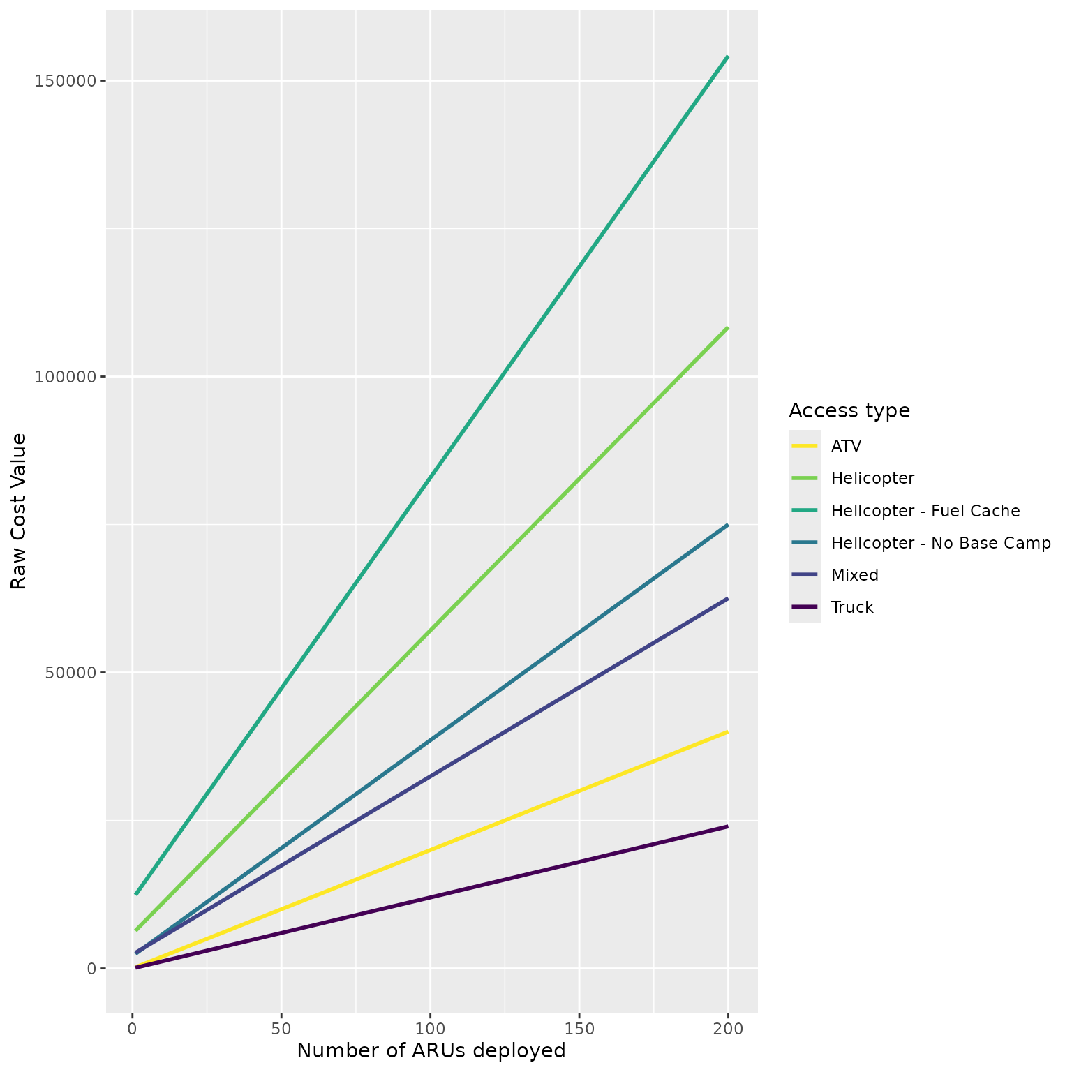

The cost of deploying a given number of ARUs in a Study Area by ATV, Truck, Helicopter, or a mixed method. The helicopter includes, with a base camp (‘Helicopter’; 100km from base camp to study area, 250 from study area to airport, and 200 km from airport to base camp), with no basecamp required (100km from base camp to study area, 130 from study area to airport, and 200 km from airport to base camp), and with a base camp and secondary fuel cach required (200km from base camp to study area, 250 km from study area to airport, and 200 km from airport to base camp). The ‘Mixed’ method involves 1/3 of truck, ATV, and Helicopter access types to survey the area.

  # scale_y_continuous(trans = 'log1p')

ggplot(cost_test, aes(narus,scLogCost, colour = StudyAreaID )) + 
  geom_line(size = 1) +
  scale_colour_viridis_d(direction = -1) +
  labs(colour = "Access type", x = "Number of ARUs deployed", y = "Scaled Log Cost")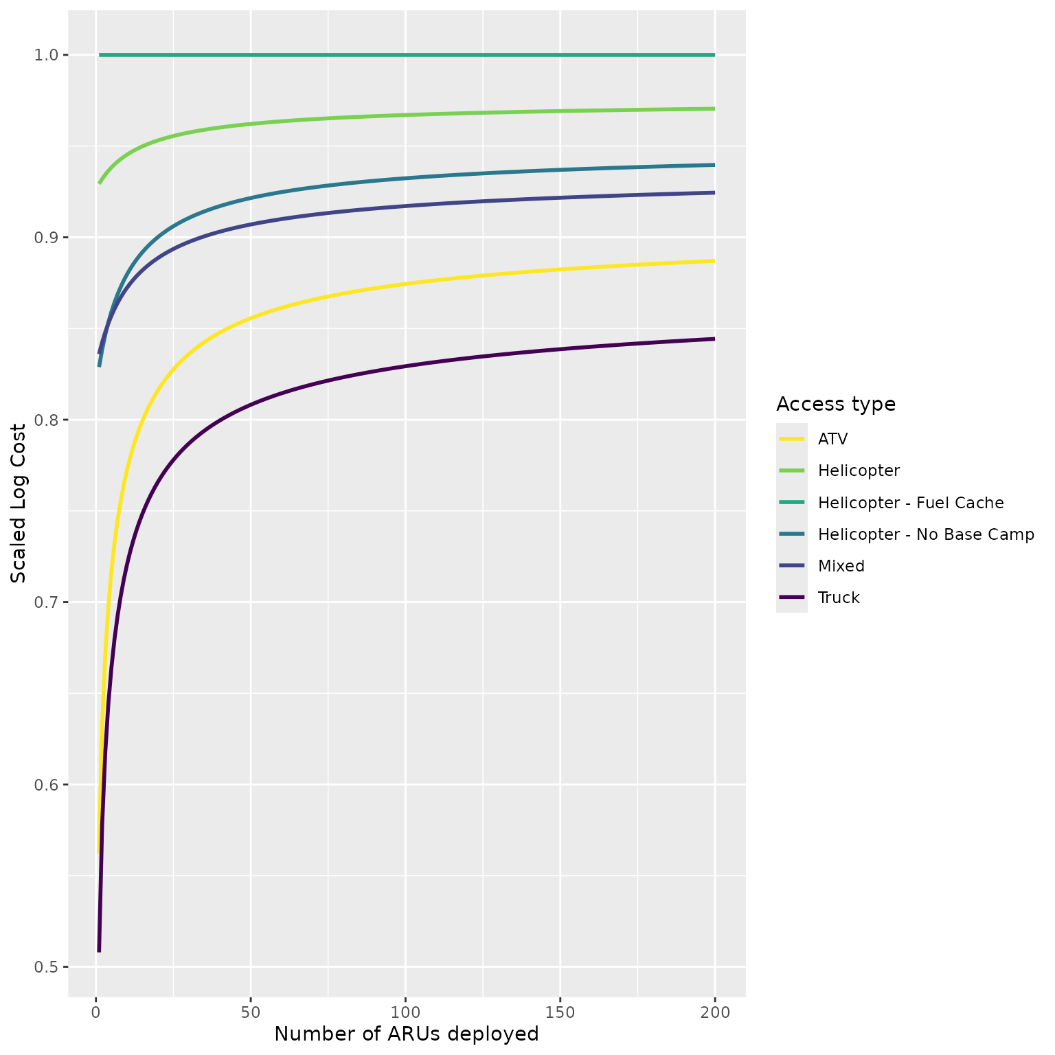

The same calculation shown in the figure above but now cost is shown as the cost relative to the most expensive access type for each ARU deployment size (here it is ‘Helicopter - Fuel Cache’ for all ARU numbers). The scaled cost is calculated as the raw cost divided by the maximum raw cost for that ARU number.

Baseline variables

BASSr::cost_vars %>% as_tibble() %>% 
  dplyr::select(-helicopter_airport_cost_per_l) %>% 
  pivot_longer(names_to = "Variable", values_to = "Value", cols = everything()) %>% 
  # BASSr::cost_vars$helicopter_airport_cost_per_l
  knitr::kable()

Variable	Value
truck_cost_per_day	600
truck_n_crews	2
truck_arus_per_crew_per_day	5
atv_cost_per_day	1200
atv_n_crews	2
atv_arus_per_crew_per_day	3
helicopter_cost_per_hour	1250
helicopter_max_km_from_base	150
helicopter_base_setup_cost_per_km	9
helicopter_l_per_hour	160
helicopter_crew_size	4
helicopter_aru_per_person_per_day	5
helicopter_relocation_speed	180
helicopter_base_cost_per_l	5
helicopter_2nd_base_cost_per_l	10
helicopter_hours_flying_within_sa_per_day	5
truck_cost_per_day	600
truck_n_crews	2
truck_arus_per_crew_per_day	5
atv_cost_per_day	1200
atv_n_crews	2
atv_arus_per_crew_per_day	3
helicopter_cost_per_hour	1250
helicopter_max_km_from_base	150
helicopter_base_setup_cost_per_km	9
helicopter_l_per_hour	160
helicopter_crew_size	4
helicopter_aru_per_person_per_day	5
helicopter_relocation_speed	180
helicopter_base_cost_per_l	5
helicopter_2nd_base_cost_per_l	10
helicopter_hours_flying_within_sa_per_day	5
truck_cost_per_day	600
truck_n_crews	2
truck_arus_per_crew_per_day	5
atv_cost_per_day	1200
atv_n_crews	2
atv_arus_per_crew_per_day	3
helicopter_cost_per_hour	1250
helicopter_max_km_from_base	150
helicopter_base_setup_cost_per_km	9
helicopter_l_per_hour	160
helicopter_crew_size	4
helicopter_aru_per_person_per_day	5
helicopter_relocation_speed	180
helicopter_base_cost_per_l	5
helicopter_2nd_base_cost_per_l	10
helicopter_hours_flying_within_sa_per_day	5

With current version, you can adjust cost of fuel based on airport type

  BASSr::cost_vars$helicopter_airport_cost_per_l %>% 
  knitr::kable()

AirportType	lCost
Highway	1.3
Secondary	1.5
Remote	2.0

Vignette Author

2025-06-20

Cost model parts

Baseline variables