## Linking to GEOS 3.12.1, GDAL 3.8.4, PROJ 9.4.0; sf_use_s2() is TRUE##
## Attaching package: 'dplyr'## The following objects are masked from 'package:stats':
##
## filter, lag## The following objects are masked from 'package:base':
##
## intersect, setdiff, setequal, unionSetup
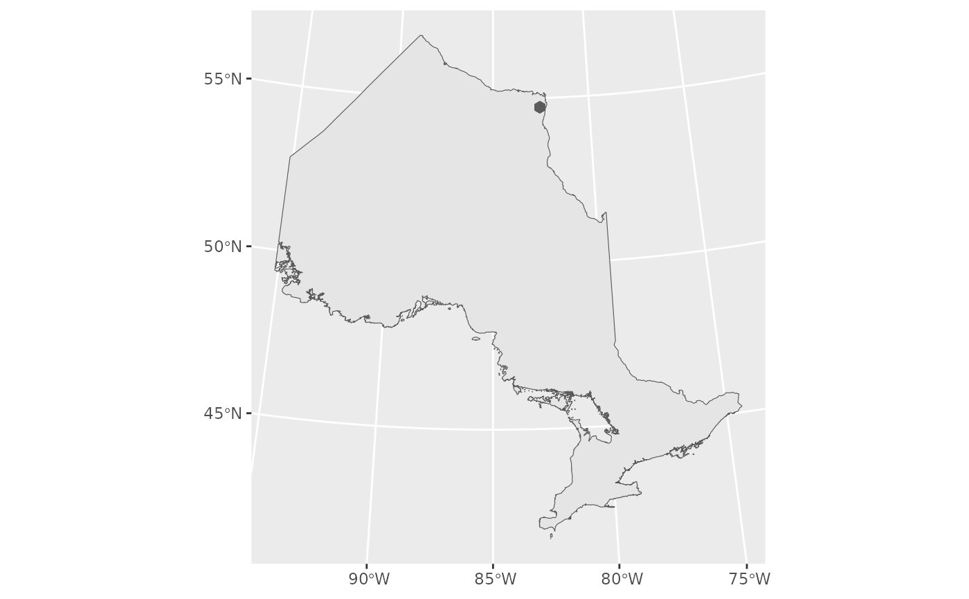
- Get spatial data - Hexagonal grid (primary spatial units - PSU) with land cover characteristics for each hex
- Get cost data
- Run
full_BASS_run()
1. Spatial Data
- Spatial data frame (sf object) with
- Columns Cell/Hex ID (e.g.,
ET_Index,hex_id) - Columns defining land cover (e.g., CORINE land cover CLC
CLC15_1)
- Columns Cell/Hex ID (e.g.,
- This must be either POINT or (MULTI)POLYGON (will be converted to points)
Land cover characteristics should not be percentages, but should be XXXX?
Clean up hex data
ont_hex <- clean_land_cover(StudyArea_hexes$landcover, pattern = "LC")## ℹ Renaming land cover columns
## • From: LC02, LC05, LC08, LC10, LC12, LC13, LC14, LC01, LC18, LC06, LC16, LC17, LC11
## • To: LC02, LC05, LC08, LC10, LC12, LC13, LC14, LC01, LC18, LC06, LC16, LC17, LC11Where are we looking?
What does this landscape look like specifically? (Thinking about LC01)
ggplot() +
  geom_sf(data = ont_hex, aes(fill = LC01)) +
  scale_fill_viridis_c()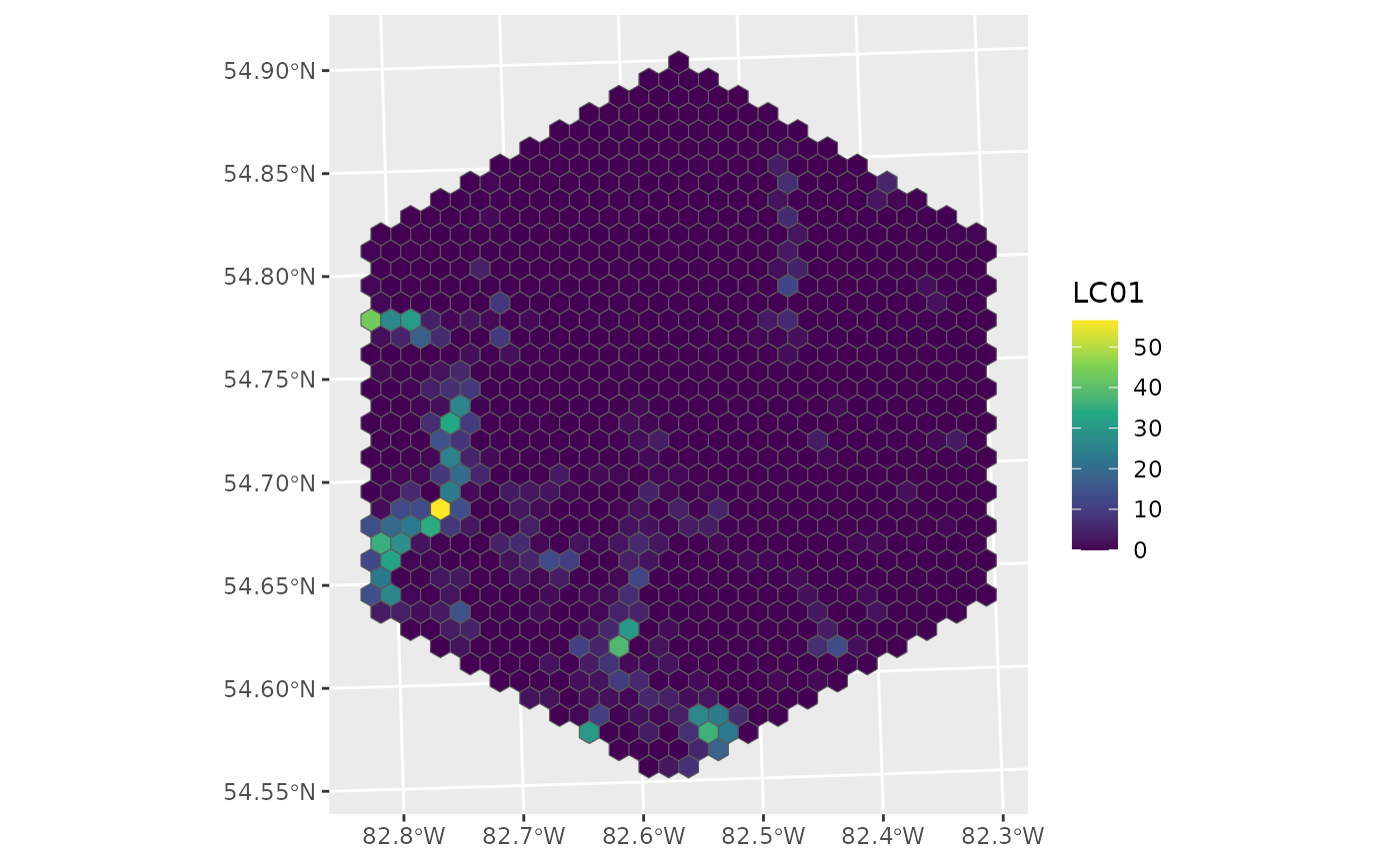
Basic Run
d <- full_BASS_run(land_hex = ont_hex,
                   num_runs = 10,
                   n_samples = 3,
                   hex_id = SampleUnitID)
## ℹ Spatial object land_hex should be POINTs not POLYGONs
## • Don't worry, I'll fix it!
## • Assuming constant attributes and using centroids as points
## ℹ Finished GRTS draw of 10 runs and 3 samples## Warning: ! Values across LC columns sum to 100 or 1,
## ℹ Check to be sure you have not input inputed percentages into your values.
## ✖ Using percentages will not calculate accurate benefit values.
ggplot(data = d, aes(colour = benefit)) +
geom_sf(size = 2) +
labs(colour = "Benefit") +
scale_colour_viridis_c()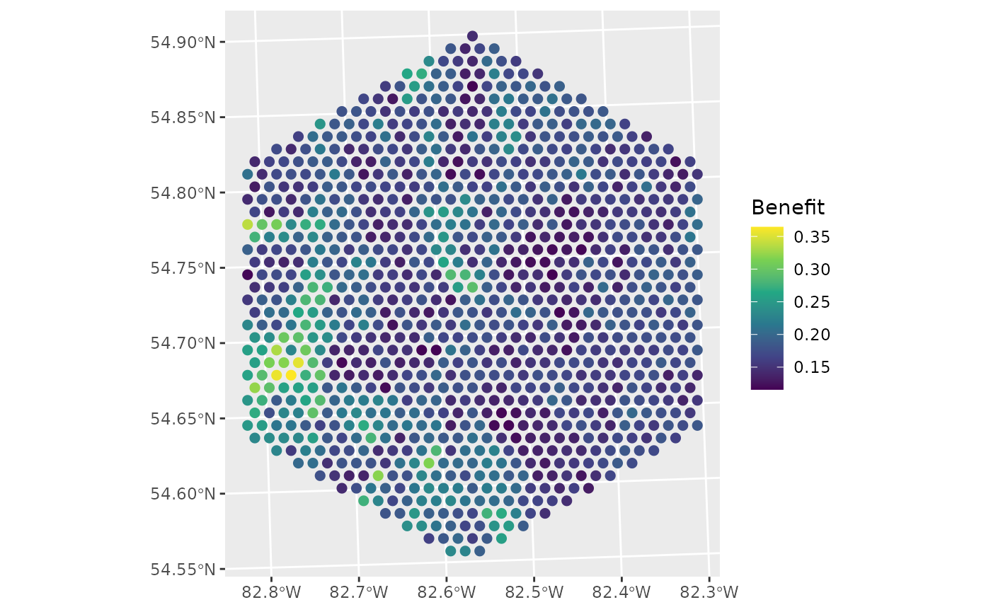
# For pretty plotting
d_hex <- left_join(ont_hex, st_drop_geometry(d), by = "SampleUnitID")
ggplot(data = d_hex, aes(fill = benefit)) +
geom_sf() +
labs(fill = "Benefit") +
scale_fill_viridis_c()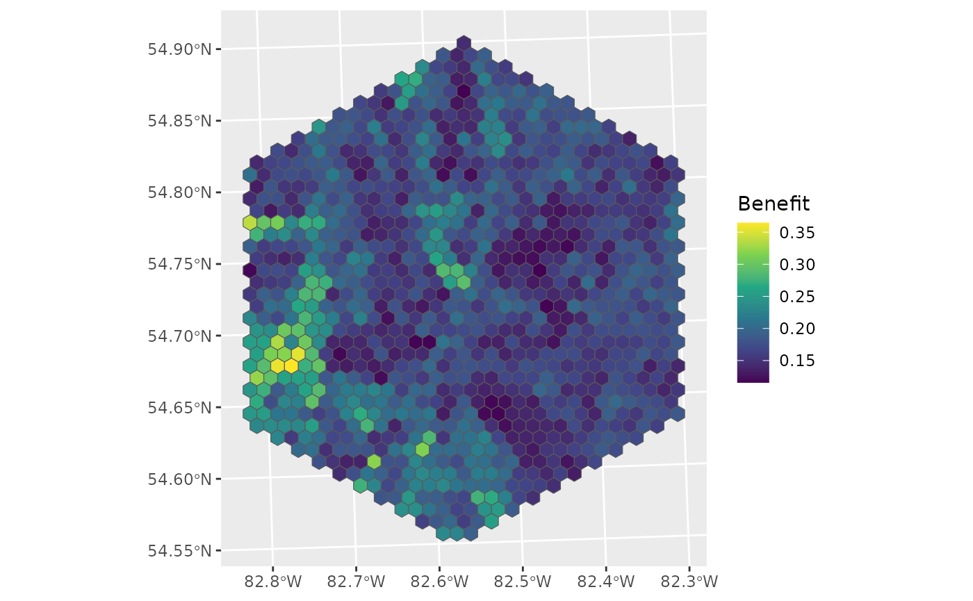
Including Costs
costs <- StudyArea_hexes$cost
d <- full_BASS_run(land_hex = ont_hex,
num_runs = 10,
n_samples = 3,
costs = costs,
hex_id = SampleUnitID,
seed = 1234)## ℹ Spatial object land_hex should be POINTs not POLYGONs
## • Don't worry, I'll fix it!
## • Assuming constant attributes and using centroids as points
## ℹ Finished GRTS draw of 10 runs and 3 samples## Warning: ! Values across LC columns sum to 100 or 1,
## ℹ Check to be sure you have not input inputed percentages into your values.
## ✖ Using percentages will not calculate accurate benefit values.
d_hex <- left_join(ont_hex, st_drop_geometry(d), by = "SampleUnitID")
ggplot(data = d_hex, aes(fill = inclpr)) +
geom_sf() +
labs(fill = "Inclusion\nProbability") +
scale_fill_viridis_c()
Perhaps we should omit sites in water. These are identified in the
costs data by TRUE/FALSEs in the
column INLAKE and can be omitted by using the
omit_flag argument.
d <- full_BASS_run(land_hex = ont_hex,
num_runs = 10,
n_samples = 3,
costs = costs,
hex_id = SampleUnitID,
omit_flag = INLAKE,
seed = 1234)## ℹ Spatial object land_hex should be POINTs not POLYGONs
## • Don't worry, I'll fix it!
## • Assuming constant attributes and using centroids as points
## ℹ Finished GRTS draw of 10 runs and 3 samples## Warning: ! Values across LC columns sum to 100 or 1,
## ℹ Check to be sure you have not input inputed percentages into your values.
## ✖ Using percentages will not calculate accurate benefit values.
d_hex <- left_join(ont_hex, st_drop_geometry(d), by = "SampleUnitID")
ggplot(data = d_hex, aes(fill = inclpr)) +
geom_sf() +
labs(fill = "Inclusion\nProbability") +
scale_fill_viridis_c()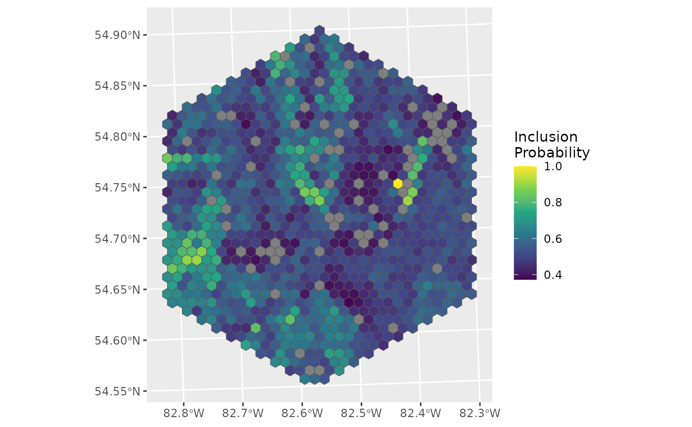
The grey hexes have been omitted.
What if the costs of that highly beneficial point was much higher?
which.max(d$inclpr)## [1] 599
high_cost <- costs
high_cost$RawCost[559] <- high_cost$RawCost[559] * 100
d <- full_BASS_run(land_hex = ont_hex,
num_runs = 10,
n_samples = 3,
costs = high_cost,
hex_id = SampleUnitID)## ℹ Spatial object land_hex should be POINTs not POLYGONs
## • Don't worry, I'll fix it!
## • Assuming constant attributes and using centroids as points
## ℹ Finished GRTS draw of 10 runs and 3 samples## Warning: ! Values across LC columns sum to 100 or 1,
## ℹ Check to be sure you have not input inputed percentages into your values.
## ✖ Using percentages will not calculate accurate benefit values.
d_hex <- left_join(ont_hex, st_drop_geometry(d), by = "SampleUnitID")
ggplot(data = d_hex, aes(fill = inclpr)) +
geom_sf() +
labs(fill = "Inclusion\nProbability") +
scale_fill_viridis_c()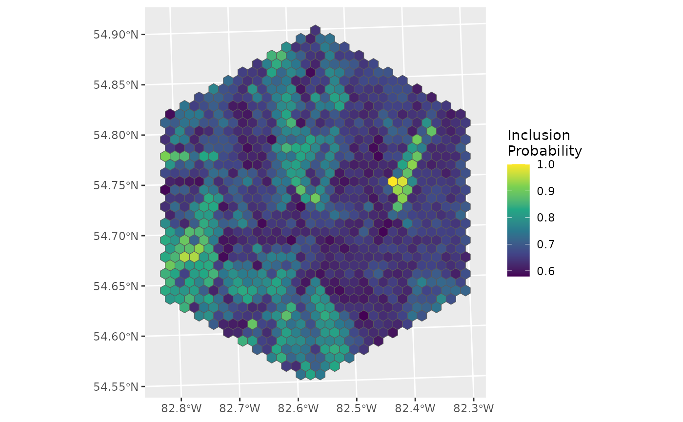
Not a great option any more.
Runs by ‘hand’
on_hex <- clean_land_cover(StudyArea_hexes$landcover, pattern = "LC")## ℹ Renaming land cover columns
## • From: LC02, LC05, LC08, LC10, LC12, LC13, LC14, LC01, LC18, LC06, LC16, LC17, LC11
## • To: LC02, LC05, LC08, LC10, LC12, LC13, LC14, LC01, LC18, LC06, LC16, LC17, LC11
samples <- draw_random_samples(on_hex, num_runs = 10, n_samples = 3,
seed = 1234)## ℹ Spatial object land_hex should be POINTs not POLYGONs
## • Don't worry, I'll fix it!
## • Assuming constant attributes and using centroids as points
## ℹ Finished GRTS draw of 10 runs and 3 samples
benefit <- calculate_benefit(on_hex, samples, hex_id = SampleUnitID)## ℹ Spatial object land_hex should be POINTs not POLYGONs
## • Don't worry, I'll fix it!
## • Assuming constant attributes and using centroids as points## Warning: ! Values across LC columns sum to 100 or 1,
## ℹ Check to be sure you have not input inputed percentages into your values.
## ✖ Using percentages will not calculate accurate benefit values.
inc_prob <- calculate_inclusion_probs(benefit,
costs = costs,
hex_id = SampleUnitID)
d_hex <- left_join(on_hex, st_drop_geometry(inc_prob), by = "SampleUnitID")
ggplot(data = d_hex, aes(fill = inclpr)) +
geom_sf() +
labs(fill = "Inclusion\nProbability") +
scale_fill_viridis_c()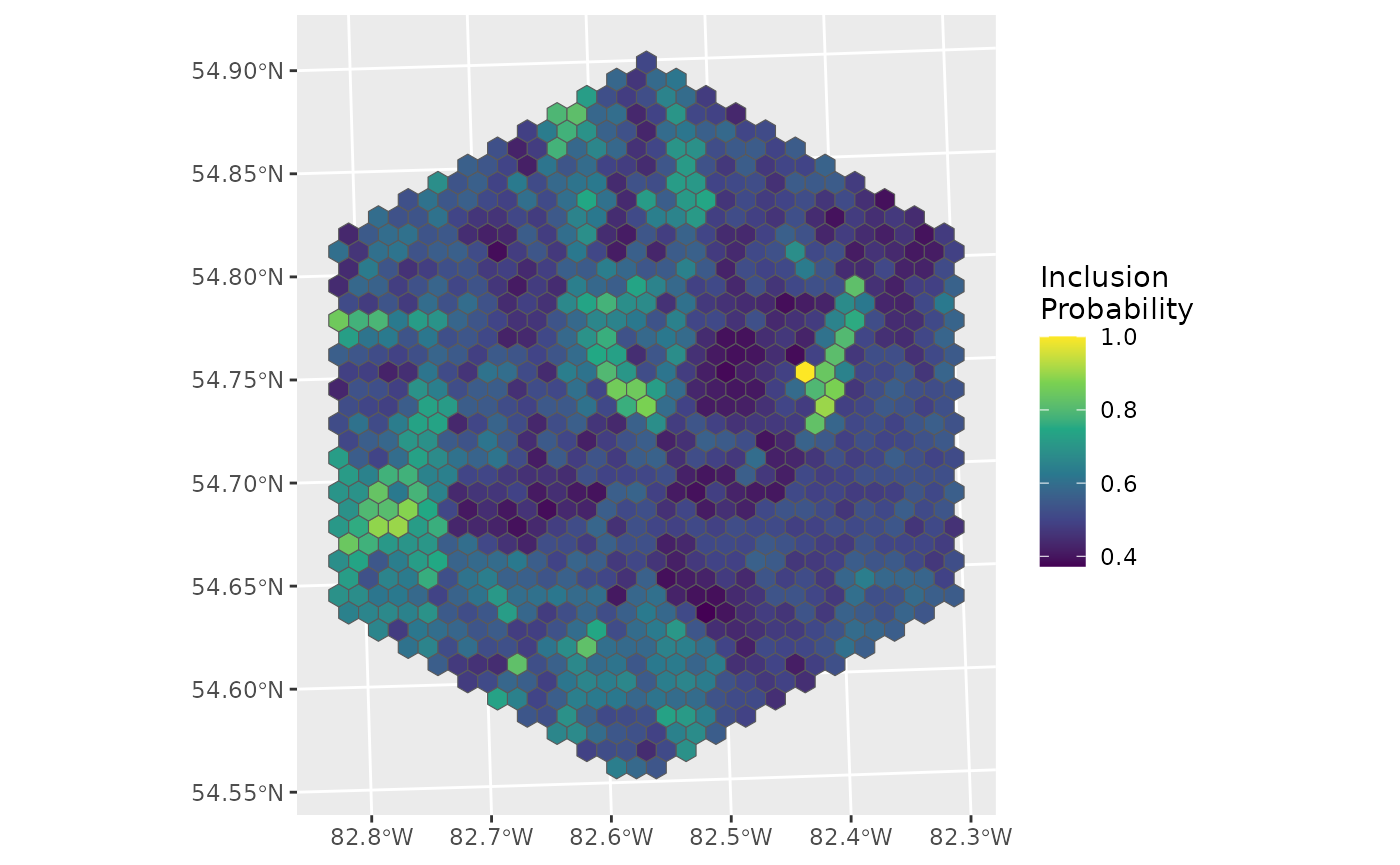
Alternative pipe
ont_hex <- clean_land_cover(StudyArea_hexes$landcover, pattern = "LC")## ℹ Renaming land cover columns
## • From: LC02, LC05, LC08, LC10, LC12, LC13, LC14, LC01, LC18, LC06, LC16, LC17, LC11
## • To: LC02, LC05, LC08, LC10, LC12, LC13, LC14, LC01, LC18, LC06, LC16, LC17, LC11
final <- ont_hex |>
draw_random_samples(num_runs = 10, n_samples = 3) %>%
calculate_benefit(ont_hex, samples = ., hex_id = SampleUnitID) %>%
calculate_inclusion_probs(costs = costs, hex_id = SampleUnitID)## ℹ Spatial object land_hex should be POINTs not POLYGONs
## • Don't worry, I'll fix it!
## • Assuming constant attributes and using centroids as points
## ℹ Spatial object land_hex should be POINTs not POLYGONs
## • Don't worry, I'll fix it!
## • Assuming constant attributes and using centroids as points
## ℹ Finished GRTS draw of 10 runs and 3 samples
## Warning: ! Values across LC columns sum to 100 or 1,
## ℹ Check to be sure you have not input inputed percentages into your values.
## ✖ Using percentages will not calculate accurate benefit values.Selection probabilities
Simple selection
Here we’ll sample 12 sites with a 20% over sample, resulting in a total of 14 sites selected.
g <- ggplot() +
  geom_sf(data = ont_hex, fill = "white") +
  geom_sf(data = final, colour = "grey70")

g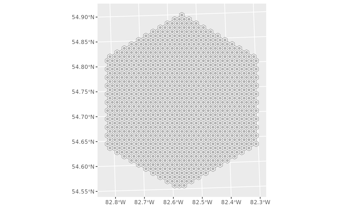
sel <- run_grts_on_BASS(probs = final,
                        num_runs = 1,
                        nARUs = 12,
                        os = 0.2)

sel_plot <- bind_rows(sel[["sites_base"]],
                      sel[["sites_over"]])

g +
  geom_sf(data = sel_plot, aes(colour = siteuse), size = 5) +
  scale_colour_viridis_d(name = "Type of\nsites sampled", end = 0.7)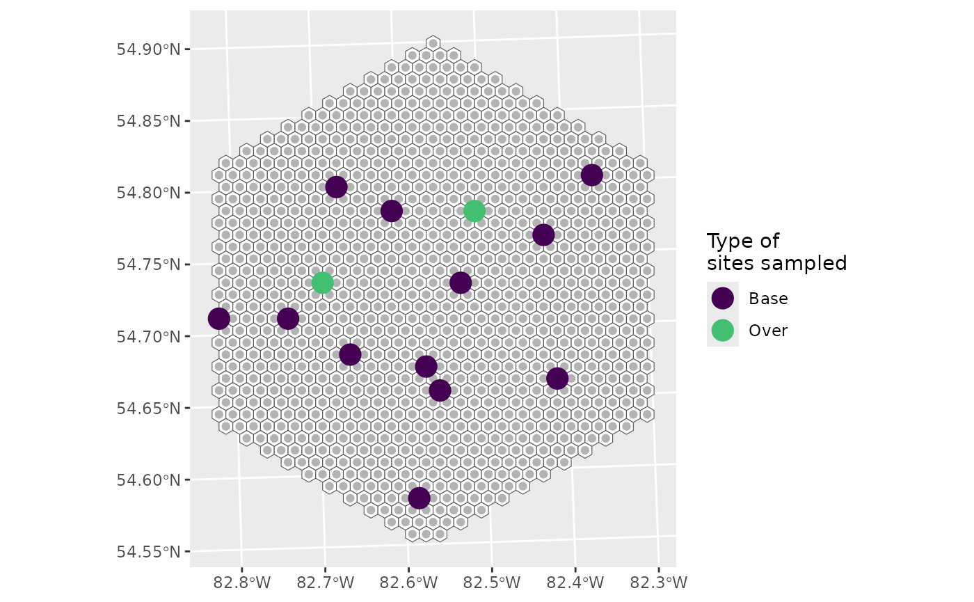
Stratified selection
First let’s create a dummy stratification and add it to our hexes for plotting
final <- mutate(final, strat = c(rep("A", 300), rep("B", 703)))
ont_hex_strat <- select(final, "SampleUnitID", "strat") |>
  st_drop_geometry() |>
  left_join(ont_hex, y = _, by = "SampleUnitID")

g <- ggplot() +
  geom_sf(data = ont_hex_strat, aes(fill = strat), alpha = 0.4) +
  geom_sf(data = final, colour = "grey70")
g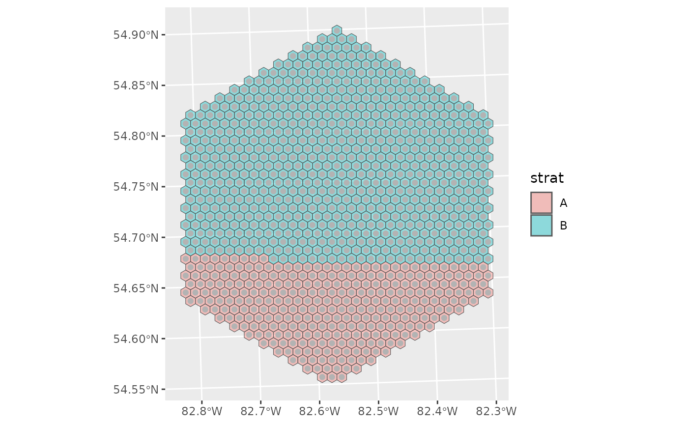
Now we’ll define how we want to sample these two strata.
Let’s assume we don’t really care about habitat A, so we don’t want to sample that one very much.
nARUs <- list("A" = 2, "B" = 50)

sel <- run_grts_on_BASS(probs = final,
                        num_runs = 1,
                        stratum_id = strat,
                        nARUs = nARUs,
                        os = 0.2)

sel_plot <- bind_rows(sel[["sites_base"]],
                      sel[["sites_over"]])

g +
  geom_sf(data = sel_plot, aes(colour = siteuse), size = 5) +
  scale_colour_viridis_d(name = "Type of\nsites sampled", end = 0.7)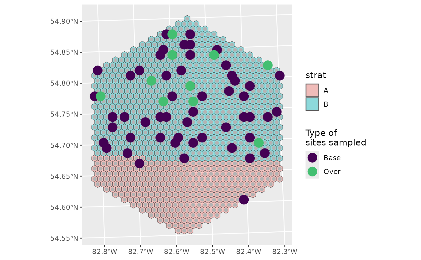
You can see that we’ve sampled much more of B than A, and that there are no over samples in A, which makes sense:
0.2 * 2 = 0.4 which rounds down to 0
If we wanted an over sample for A, we could define specific over sample amounts instead.
nARUs <- list("A" = 2, "B" = 50)
os <- list("A" = 1, "B" = 4)

sel <- run_grts_on_BASS(probs = final,
                        num_runs = 1,
                        stratum_id = strat,
                        nARUs = nARUs,
                        os = os,
                        seed = 123)

sel_plot <- bind_rows(sel[["sites_base"]],
                      sel[["sites_over"]])

g +
  geom_sf(data = sel_plot, aes(colour = siteuse), size = 5) +
  scale_colour_viridis_d(name = "Type of\nsites sampled", end = 0.7)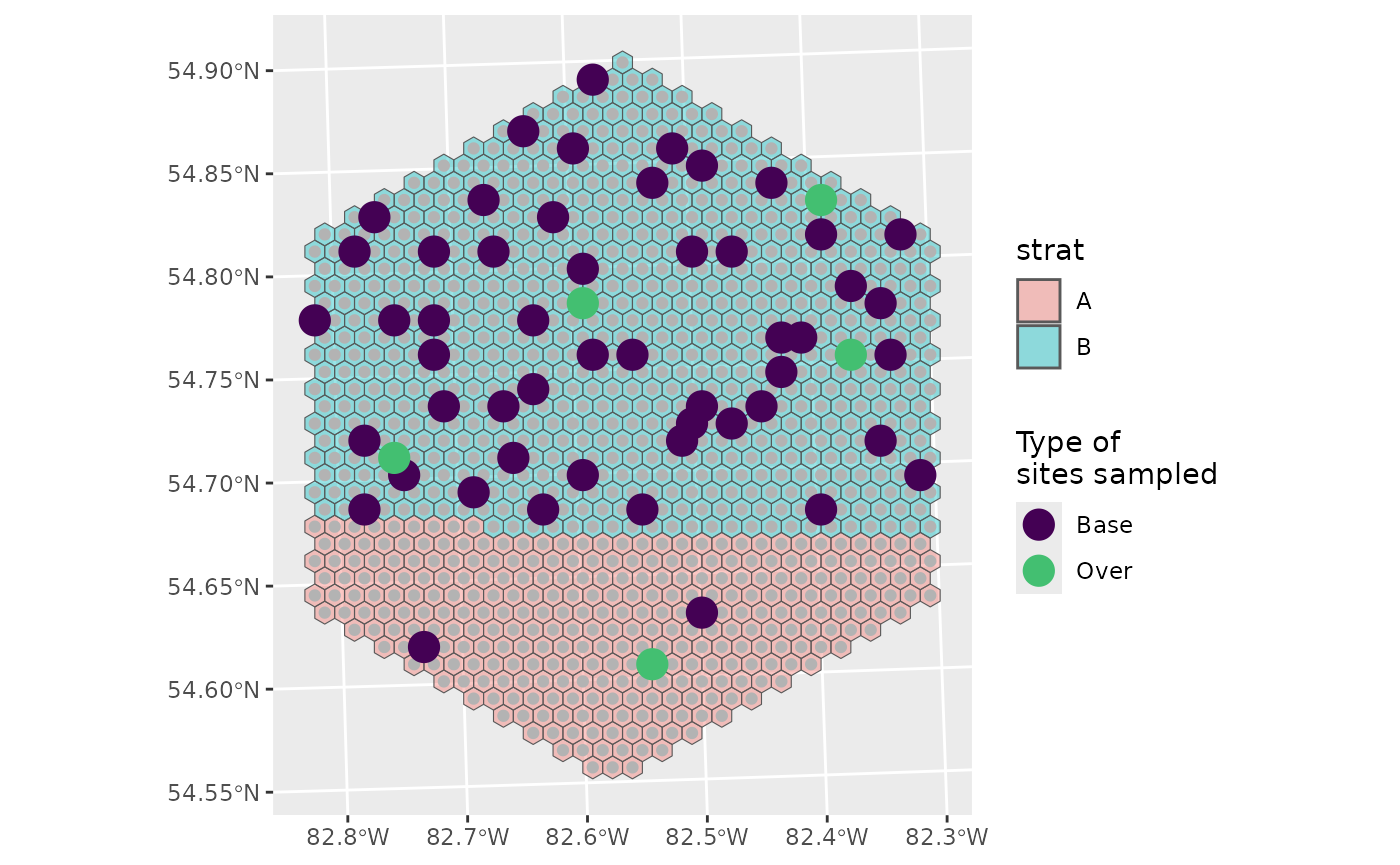
Alternatively at this point (and especially with more strata) it might be easier to supply a data frame rather than a series of lists.
nARUs <- data.frame(n = c(2, 50),
                    strat = c("A", "B"),
                    n_os = c(1, 4))

sel <- run_grts_on_BASS(probs = final,
                        num_runs = 1,
                        stratum_id = strat,
                        nARUs = nARUs,
                        seed = 123)

sel_plot <- bind_rows(sel[["sites_base"]],
                      sel[["sites_over"]])

g +
  geom_sf(data = sel_plot, aes(colour = siteuse), size = 5) +
  scale_colour_viridis_d(name = "Type of\nsites sampled", end = 0.7)